Plot a population pyramid (age-sex) from a dataframe.

age_pyramid(
  data,
  age_group = "age_group",
  split_by = "sex",
  stack_by = NULL,
  count = NULL,
  proportional = FALSE,
  na.rm = TRUE,
  show_midpoint = TRUE,
  vertical_lines = FALSE,
  horizontal_lines = TRUE,
  pyramid = TRUE,
  pal = NULL
)

Arguments

data	Your dataframe (e.g. linelist)
age_group	the name of a column in the data frame that defines the age group categories. Defaults to "age_group"
split_by	the name of a column in the data frame that defines the the bivariate column. Defaults to "sex". See NOTE
stack_by	the name of the column in the data frame to use for shading the bars. Defaults to `NULL` which will shade the bars by the `split_by` variable.
count	for pre-computed data the name of the column in the data frame for the values of the bars. If this represents proportions, the values should be within [0, 1].
proportional	If `TRUE`, bars will represent proportions of cases out of the entire population. Otherwise (`FALSE`, default), bars represent case counts
na.rm	If `TRUE`, this removes NA counts from the age groups. Defaults to `TRUE`.
show_midpoint	When `TRUE` (default), a dashed vertical line will be added to each of the age bars showing the halfway point for the un-stratified age group. When `FALSE`, no halfway point is marked.
vertical_lines	If you would like to add dashed vertical lines to help visual interpretation of numbers. Default is to not show (`FALSE`), to turn on write `TRUE`.
horizontal_lines	If `TRUE` (default), horizontal dashed lines will appear behind the bars of the pyramid
pyramid	if `TRUE`, then binary `split_by` variables will result in a population pyramid (non-binary variables cannot form a pyramid). If `FALSE`, a pyramid will not form.
pal	a color palette function or vector of colors to be passed to `ggplot2::scale_fill_manual()` defaults to the first "qual" palette from `ggplot2::scale_fill_brewer()`.

Note

If the split_by variable is bivariate (e.g. an indicator for a specific symptom), then the result will show up as a pyramid, otherwise, it will be presented as a facetted barplot with with empty bars in the background indicating the range of the un-facetted data set. Values of split_by will show up as labels at top of each facet.

Examples


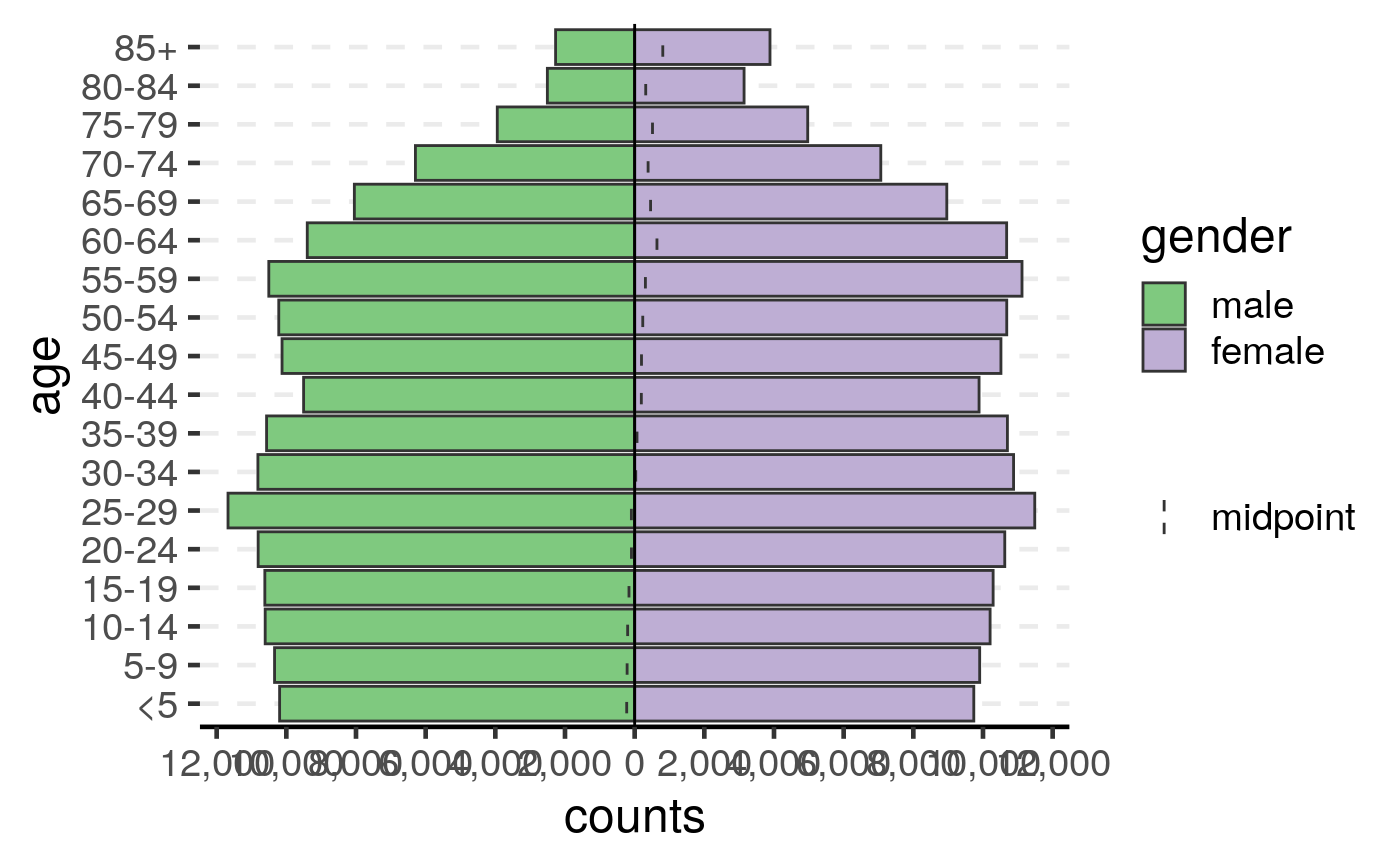
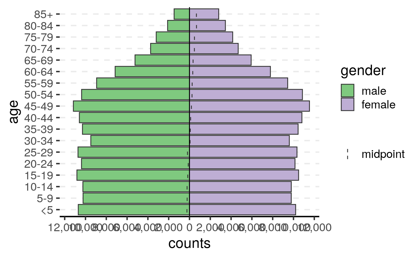
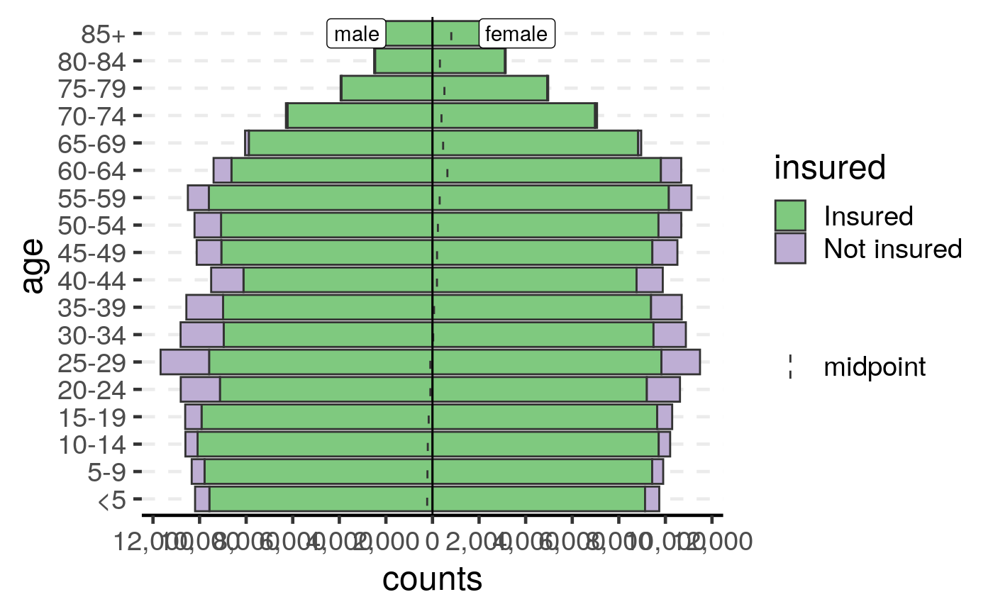
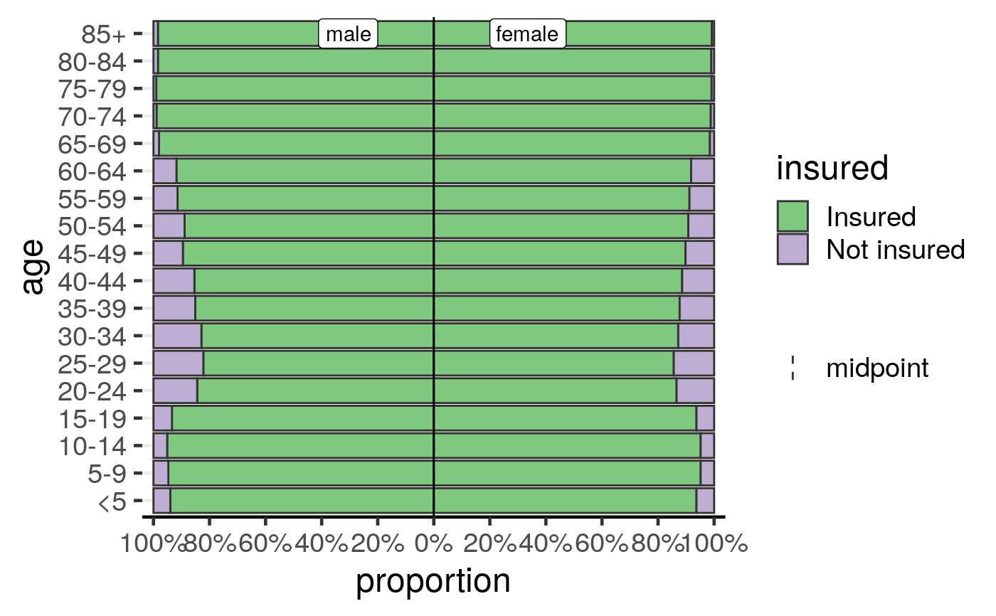
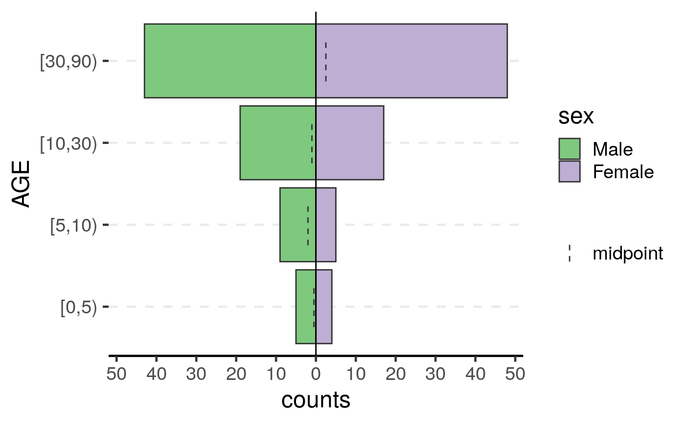
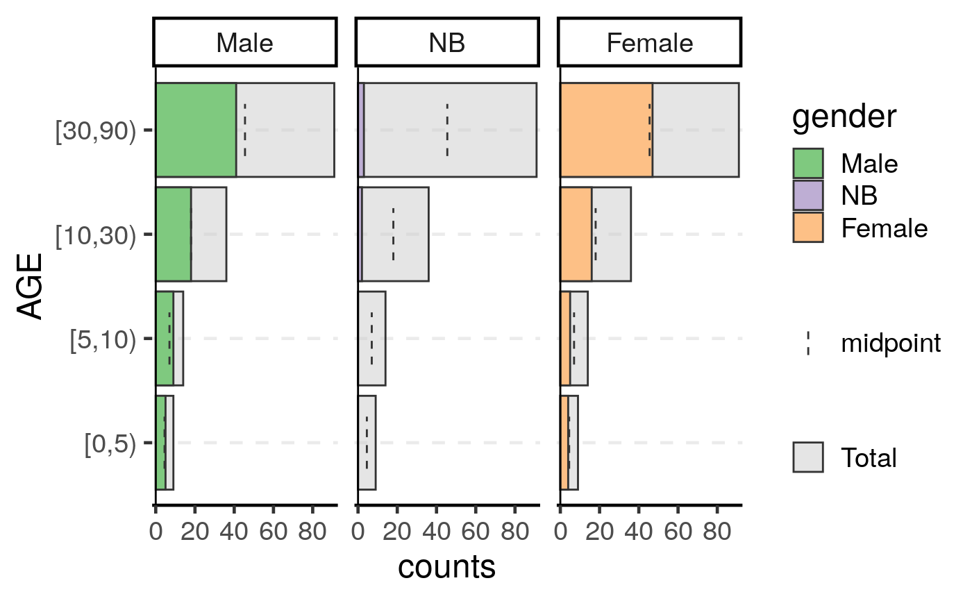
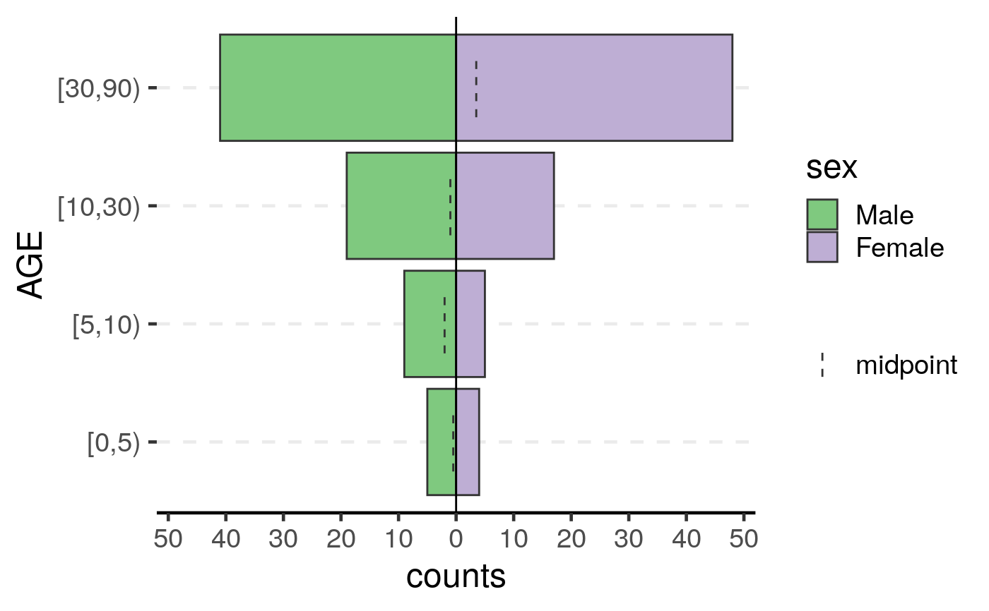
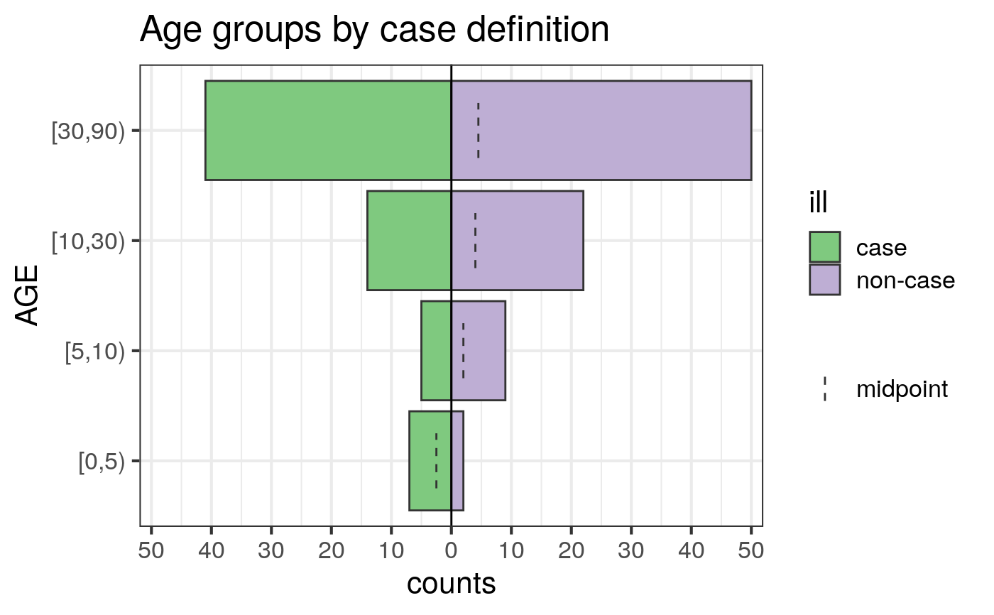
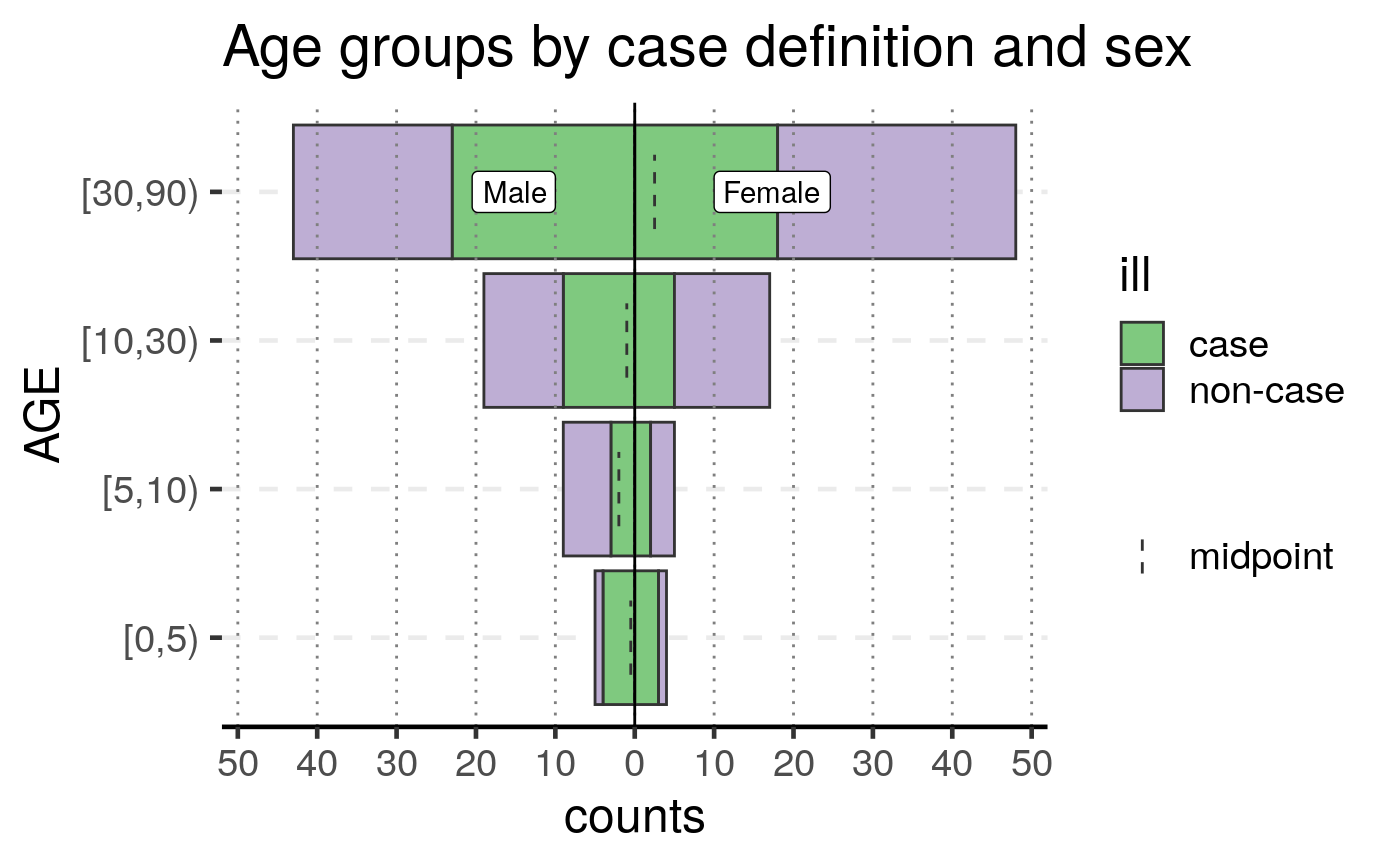
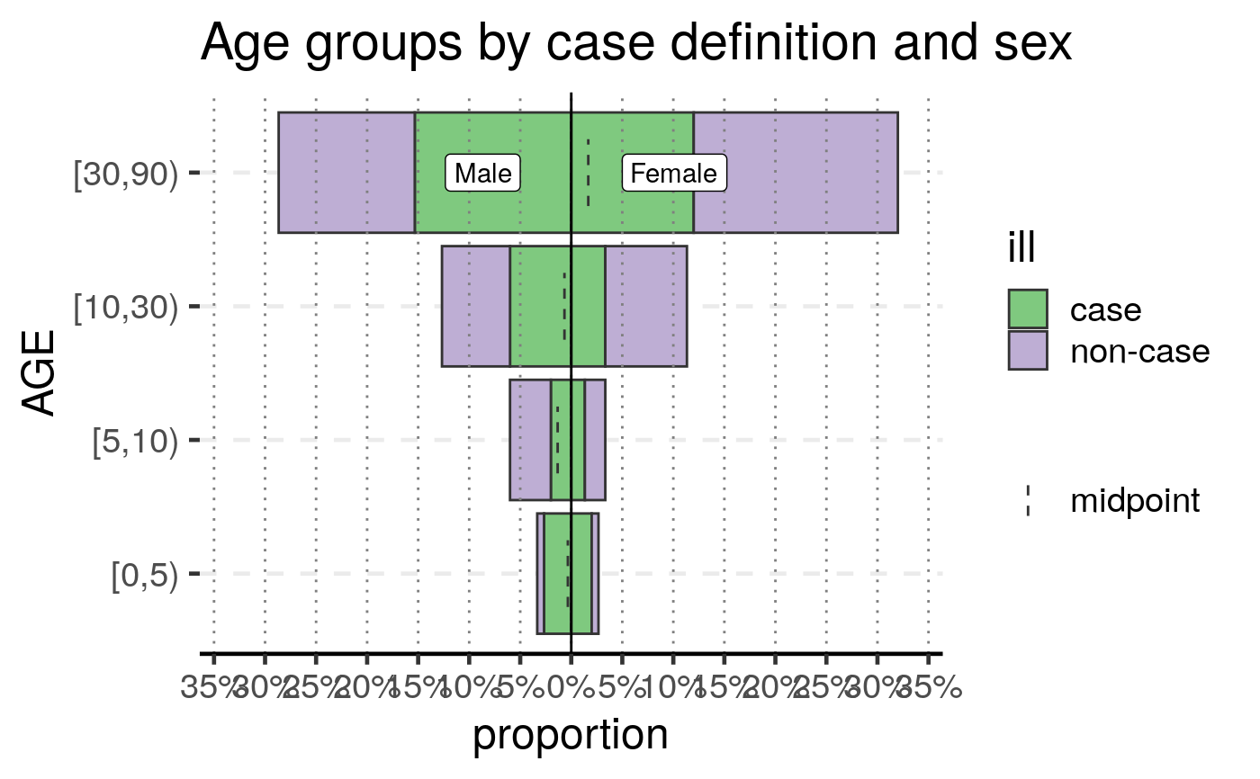
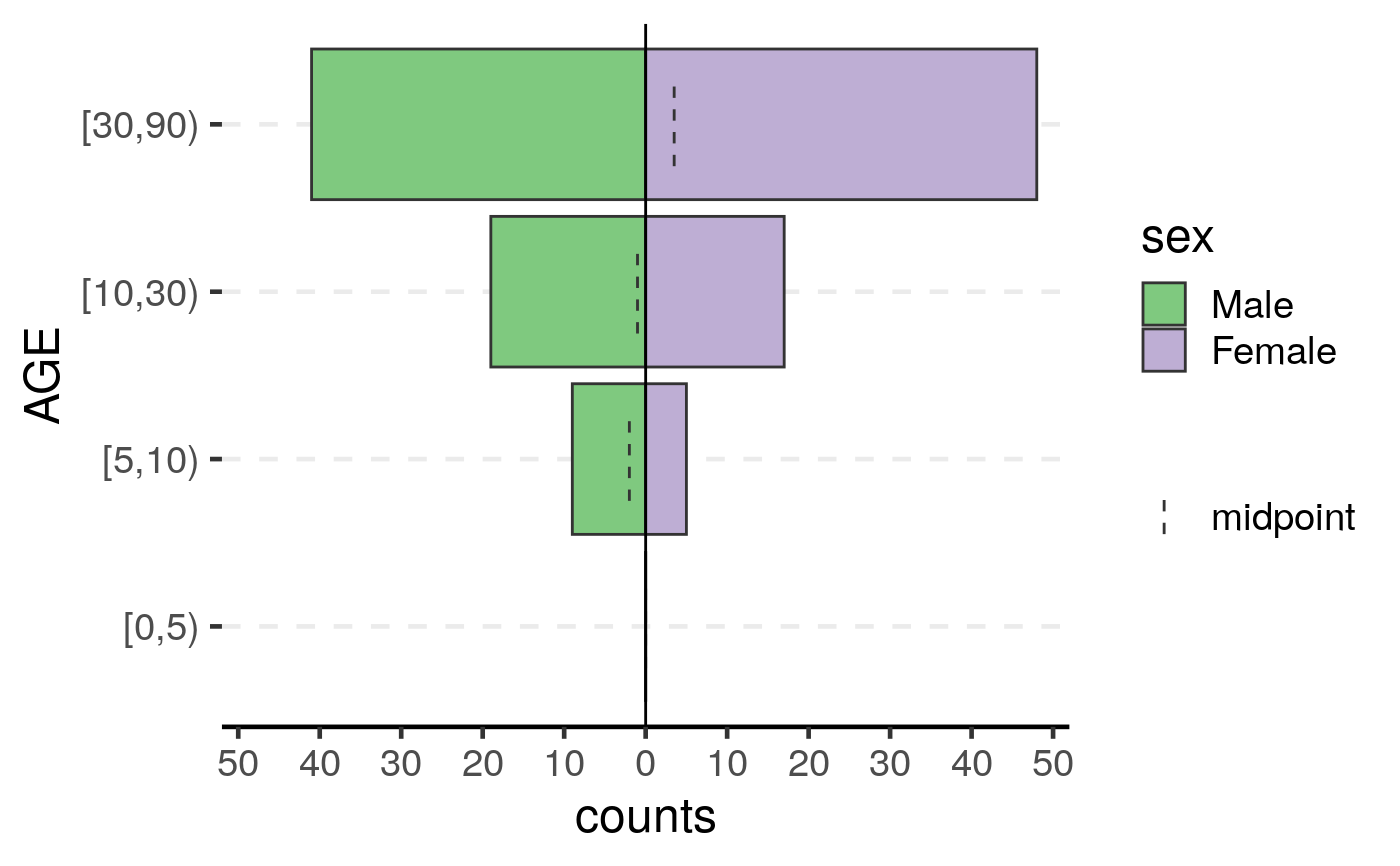
library(ggplot2)
old <- theme_set(theme_classic(base_size = 18))

# with pre-computed data ----------------------------------------------------
# 2018/2008 US census data by age and gender
data(us_2018)
data(us_2008)
age_pyramid(us_2018, age_group = age, split_by = gender, count = count)
age_pyramid(us_2008, age_group = age, split_by = gender, count = count)

# 2018 US census data by age, gender, and insurance status
data(us_ins_2018)
age_pyramid(us_ins_2018,
  age_group = age,
  split_by = gender,
  stack_by = insured,
  count = count
)
us_ins_2018$prop <- us_ins_2018$percent/100
age_pyramid(us_ins_2018,
  age_group = age,
  split_by = gender,
  stack_by = insured,
  count = prop,
  proportion = TRUE
)

# from linelist data --------------------------------------------------------
set.seed(2018 - 01 - 15)
ages <- cut(sample(80, 150, replace = TRUE),
  breaks = c(0, 5, 10, 30, 90), right = FALSE
)
sex <- sample(c("Female", "Male"), 150, replace = TRUE)
gender <- sex
gender[sample(5)] <- "NB"
ill <- sample(c("case", "non-case"), 150, replace = TRUE)
dat <- data.frame(
  AGE = ages,
  sex = factor(sex, c("Male", "Female")),
  gender = factor(gender, c("Male", "NB", "Female")),
  ill = ill,
  stringsAsFactors = FALSE
)

# Create the age pyramid, stratifying by sex
print(ap <- age_pyramid(dat, age_group = AGE))

# Create the age pyramid, stratifying by gender, which can include non-binary
print(apg <- age_pyramid(dat, age_group = AGE, split_by = gender))

# Remove NA categories with na.rm = TRUE
dat2 <- dat
dat2[1, 1] <- NA
dat2[2, 2] <- NA
dat2[3, 3] <- NA
print(ap <- age_pyramid(dat2, age_group = AGE))
#> Warning: 2 missing rows were removed (1 values from `AGE` and 1 values from `sex`).
print(ap <- age_pyramid(dat2, age_group = AGE, na.rm = TRUE))
#> Warning: 2 missing rows were removed (1 values from `AGE` and 1 values from `sex`).

# Stratify by case definition and customize with ggplot2
ap <- age_pyramid(dat, age_group = AGE, split_by = ill) +
  theme_bw(base_size = 16) +
  labs(title = "Age groups by case definition")
print(ap)

# Stratify by multiple factors
ap <- age_pyramid(dat,
  age_group = AGE,
  split_by = sex,
  stack_by = ill,
  vertical_lines = TRUE
) +
  labs(title = "Age groups by case definition and sex")
print(ap)

# Display proportions
ap <- age_pyramid(dat,
  age_group = AGE,
  split_by = sex,
  stack_by = ill,
  proportional = TRUE,
  vertical_lines = TRUE
) +
  labs(title = "Age groups by case definition and sex")
print(ap)

# empty group levels will still be displayed
dat3 <- dat2
dat3[dat$AGE == "[0,5)", "sex"] <- NA
age_pyramid(dat3, age_group = AGE)
#> Warning: 11 missing rows were removed (1 values from `AGE` and 10 values from `sex`).
theme_set(old)